Kidney Exchange in Julia

The Kidney Donation Problem

Some of the most powerful research coming from Operations Researchers originates in the healthcare field where there are some notorious inefficiencies. If you’ve ever had a loved one in need of a life-saving transplant, this emerging research may one day become the difference between life and death for many.

To preface the subject, kidney exchanges aren’t necessarily a new idea, we’ve just never found a way to do them at scale. This project is in inspiration of this PNAS research article.

Full disclosure, I do not have a biology degree, that being said I can at least offer some information on the process of organ donation. For kidneys specifically, humans can live with only one, thus many healthy family members will step up and offer one of their’s to a related family member in need of one. The issue is, there must be a match or some compatibility in blood type from donor to patient. Without it, we run the risk of the kidney being rejected by the patient. This presents a special sort of challenge. What if a patient doesn’t have a family member with a compatible kidney? It turns out this is quite likely (25% of siblings are “exact matches”¹). Usually what happens when there isn’t a family member willing to give a kidney is that patients are put into a pool along with everyone else who doesn’t have a matching family donor. Think of this as a sort of waiting list. From here, they wait for an unrelated organ donor (generally upon death) to give them a kidney, which may or may not ever happen. Thus we introduce the kidney exchange.

Kidney Exchanges

To solve this predicament, we can introduce an exchange system. The way this works is in a sort of “I’ll scratch your back, if you scratch mine” type solution. The idea is this: we have a patient; this patient has a family member willing to give a kidney, but unable to due to incompatibility; we find another patient who is in a similar situation; we match these patient-donor pairs with each other, giving us four total people in the exchange; the donors each give a kidney to the patient in which they are not family related. The power of this approach, however, is that we increase the supply of kidneys in the system. Of course if you’re following along, this also presents a challenge of higher magnitude because now we must find a reciprocal match as opposed to a one-to-one match. Thus, we implement chains and cycles.

Chains

The idea behind chains is that with one Non-directed Donor (someone who gives their kidney altruistically or in posthumous organ donation), we can give that kidney to the first person on our kidney pool/list, and then the incompatible family member who would have liked to give them a kidney will give theirs to another patient in need. This starts a chain reaction of patients getting kidneys and donors giving theirs to those they don’t know, in exchange for their family member receiving a kidney from someone else. Chains look something like this:

Cycles

Cycles are similar to chains in their structure, the only difference is that cycles aren’t started by NDDs but rather a donor from a patient-donor pairing. Ultimately, cycles end with a donor giving up their kidney to the patient whose donor began the cycle. This looks something like this:

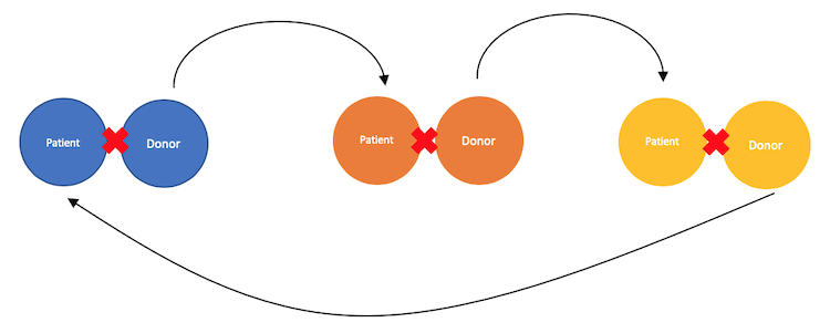
As we’ll see later, we will want to limit cycles to a maximum length of five. There are a few reasons we do this, but it is mainly because the longer a cycle is, the longer the time in which something could happen such that the patient-donor pair who began the cycle doesn’t get a kidney at the end of the cycle. Restated from above, a cycle begins when a donor from an incompatible pairing gives their kidney to someone whom they do not know, but are compatible with. The cycle completes when a donor gives their kidney to the patient who’s donor began the cycle.

Perhaps you’re wondering why have cycles at all? The reason we allow for cycles is because it gives our optimization problem some flexibility in which we can increase the number of patients who get compatible kidneys, and the kidneys in which they receive are more compatible. If we keep them short, we can give ourselves more opportunity (increase our feasible region) to match patients well.

The Data

The kidney exchange problem, in simplified terms, is an integer-programming optimization problem- nothing more. We are given a dataset of pairs in which the patient and donor are not compatible, and a score for which each pair is compatible with another pair (meaning there is a good match between the donor of one pair, and the patient of another pair). This compatibility score is the weights on our edges. The dataset looks like this:

As you can see, some pairs can perform more than one match- of course only one of these edges can have flow on it as once a patient has the kidney they need they won’t need another. Additionally, we should note that we are supplied with our NDDs of which there are only three. This tells us that we will only have three chains as chains can only be began from an NDD.

To explain the “from” and “to” columns, take the first row for example. Pairing 0’s donor can give their kidney to pairing 721’s patient in need of a kidney. This relationship may not be reciprocal, however. Meaning, 721’s donor may not be able to give their kidney to pairing 0’s patient. If 721’s donor did have a compatible kidney, there would be a row in which 721 is in the “from” column and 0 is in the “to” column, but for the sake of keeping the table simple I won’t show all the data. Rest assured, there are pairings in which pairing 0’s patient can receive a compatible kidney.

Finally, w is subscripted at _ij. For example, w_0,721 is equal to 38.

We load the data into Julia like this:

 1
 2
 3
 4
 5
 6
 7
 8
 9
10
11
12

dat = readdlm("donor-pool1.csv", ',', '\n', comments=true)

fr = dat[:,1]
to = dat[:,2]
w = dat[:,3]
N = dat[:,4]
N = N[1:3,]

V = union(fr,to)       # set of all nodes
E = collect(zip(fr,to)) # set of all edges

W = Dict( (i,j) => k for (i,j,k) in zip(fr,to,w) )  # weights on edges

The Formulation

For more detail, view the formulation in the PNAS article.

Decision Variables

In the kidney exchange problem, we want to maximize the compatibility between all patients and their newly matched donors. We achieve this through mathematical optimization which seeks to maximize our objective (patients treated and the corresponding compatibility) while remaining within constraints which we shall outline below. To do this, our optimizer will determine the pairs that should match with each other, which we will define as a decision variable.

If you’ve ever done an optimization problem, this may seem somewhat familiar. As with any optimization problem, we define our decision variables first. In terms of our problem, decision variables are the rows in which a pair in the “from” column should give its kidney to the patient in the “to” column. We can define this variable as y.

• y_ij is a binary variable. If a donor in the “from” pairing gives their kidney to a patient in the “to” pairing, this variable is set to 1. For example, if pair 0’s donor gives their kidney to pair 721’s patient, y_{0, 721} will be 1. The i and j represent the “from” and “to” pairs that are involved in the transplant.
• We also define a couple additional variables to set flow in and flow out. We will use these variables to limit the number of kidneys leaving a pair (donor gives their kidney) and the number of kidneys entering a pair (patient receives a kidney). We will set some constraints such that neither of these variables are greater than 1, but also such that if a donor gives their kidney, the incompatible patient whom they are giving the kidney for will eventually receive a compatible kidney from someone else. We can call these variables f^o and fⁱ. Each of these variables are subscripted with v. v is the set of our pairings, essentially a list from 0 to 1000 (including our NDDs). This way we can limit the flow in and out of each pairing in our dataset.

In Julia’s JuMP, we can create a model and add constraints like this:

1
2
3
4
5
6
7
8

m = Model()
set_optimizer(m, Cbc.Optimizer)

@variable(m, y[(i,j) in E], Bin)

@variable(m, f_in[i in V])

@variable(m, f_out[i in V])

We’ll use the Cbc optimizer for this problem, of course there are others.

Objective Function

To solve, we want to maximize the number of pairings that receive a kidney and the corresponding compatibility (we’d much rather match a donor to a patient with higher compatibility). In words, we maximize the sum of our weights for which a “from” pair’s donor gives a kidney to a “to” pair’s patient. To do this, we multiply the weight by the corresponding y_i,j decision variable.

1

@objective(m, Max, sum( W[(i,j)]*y[(i,j)] for (i,j) in E ))

Constraints

We have six sets of constraints. In words, these constraints are:

• We must first create two set-constraints that connect the value of our y_ij decision variable to our flow in and flow out decision variables (f^o and fⁱ).
• We need to constrain our flow in and flow out variables such that if a donor from a pairing gives a kidney, then their pairing (patient) will also receive a kidney. We should make both of these less than or equal to one. This constraint should be over the set of non-compatible pairs.
• Flow out of our NDDs should be less than or equal to one, as each NDD only has one kidney to give.

The final constraint, or more accurately set of constraints, is to keep cycles from being greater than 5.

Recursive Algorithm

If we were to merely want a solution of chains and cycles to match donors and patients with kidneys, then we’ve completed the setup. However, we want a more realistic solution and to do that we have to constrain the length of cycles. In short, we can achieve this by solving the initial optimization problem, determining what cycles are longer than 5, and adding constraints to prevent each of those cycles when we resolve.

In words, the constraint to prevent a cycle of length greater than 5 can be modeled through a sum of the y_ij’s, for which y_ij is in the cycle that is longer than 5. We make this sum less than or equal to the length of the cycle, minus 1. In Julia, we can model it like so:

1

@constraint(m, sum(y[(i,j)] for i in Cycle[z], j in Cycle[z] if in((i,j),E)) <= length(Cycle[z]) - 1)

In the algorithm, we capture all cycles greater than 5 in an array called Cycle, and we create a constraint for each cycle over 5. Step-by-step, our algorithm works like this:

1. Solve optimization problem
2. Identify cycles over 5
3. Add constraints to prevent identified cycles over 5
4. Resolve

We repeat 2-4 until we have an optimal solution with cycles all under 5. We’ve already shown how to build the initial optimization problem in Julia, so now we must show how to implement code to identify cycles, check if they’re over 5, add constraints, and resolve until we have a solution without cycles over 5.

KEP in Julia

To solve initially, we call JuMP’s optimize!() function like this:

1

JuMP.optimize!(m)

We’ll put this and everything that follows in a while loop- while all cycles aren’t under 5.

Identifying Cycles

For speed in our algorithm, we should capture the y_ij values that are equal to 1, meaning that a donor and patient have been matched. This represents our solution set.

1
2
3
4
5
6

set = []
for (i,j) in E
    if value.(y[(i,j)]) > 0
        set = union(set,i,j)
    end
end

Then we instantiate a few arrays for use in our cycle identification:

1
2
3

searched = [] # set of pairs we've searched
U = [] # capture current cycle being identified
ExtendU = set[rand(1:end)] # choose a node at random to start at

We use searched to reduce the amount of pairs we search through each time, making our algorithm faster. Additionally, we use U to capture a single cycle at a time. With ExtendU we search for and assign the next matching pair to ExtendU, and then we add ExtendU to U. Once we’ve reached the end of the cycle (when ExtendU is equal to the beginning of U) and the length of the cycle is over 5, we add it to an array called Cycle.

To begin our search of mapping each cycle, which we do through another while loop- while all pairs in our solution haven’t been matched, we randomly start somewhere within our solution set. Then, we add ExtendU to U, and reassign ExtendU to nothing.

1
2
3

while length(setdiff(set,searched))!=0
    push!(U,ExtendU)
    ExtendU = nothing

To perform our search of the next matching pair, we must introduce a for-loop to search through our solution set for the next pair. With an if statement, if we find the next pair we assign the pair to ExtendU.

1
2
3
4
5
6
7

    for j in union(U[1],setdiff(set,searched))
        if (in((U[end],j),E) && JuMP.value(y[(U[end],j)]) > 0)
            ExtendU = j
            push!(searched,ExtendU)
            break
        end
    end

There are three things that can happen after this search:

1. We find the next pair and search for the next matching pair (while we haven’t matched the entire solution set).
2. We don’t find the next matching pair. This means we’ve come to the end of a chain, because chains end with the final pair not matching with anyone (meaning their donor doesn’t give a kidney to anyone). If this happens, ExtendU will stay as nothing, so we’ll reset everything to search for cycle. There are other ways to do this, as we could start from our NDDs and find the chains and remove them from our search. This is another way in which we find many sub-chains through the way we shorten our searchable set.

1
2
3
4
5
6
7
8
9

# if we've found the end of a chain
if isnothing(ExtendU)
    print("Chain Found","\n")
    U = []
    rn = setdiff(set,searched)
    ExtendU = rn[rand(1:end)] # don't pick the same one twice..
    push!(searched,ExtendU)
    # we've found a chain!
end

3. We find the next matching pair, but it’s the same as the pair for which our cycle began, meaning we’ve found a complete cycle. If this occurs, we check if the cycle is over 5. If it is, we add it to our Cycle array to add a constraint later on to prevent it from being in our next solution. If it’s under 5, we just reset and search for the next cycle.

 1
 2
 3
 4
 5
 6
 7
 8
 9
10
11
12
13
14

# if we've found the end of a cycle
if U[1]==ExtendU
    print("Cycle Found","\n")
    # we've found a cycle, lets add it to our cycle list and create
    # a constraint, if necessary
    if length(U) > 5
        push!(Cycle,U)
        cycles_over_five = cycles_over_five + 1
    end
    U = []
    rn = setdiff(set,searched)
    ExtendU = rn[rand(1:end)]
    push!(searched,ExtendU)
end

This will repeat until every pair in our solution has been matched, whether as a part of a chain or cycle.

Notice we introduce a variable cycles_over_five. This variable will allow us to determine if our current solution has no cycles over 5. If that is the case, we’ll end the algorithm.

Add Constraints for Cycles over 5

We introduce a for-loop to add constraints for each of the cycles we identify in our solutions (remember we solve iteratively). The number of constraints will accumulate as we solve each time as Cycle is a global variable.

1
2
3
4

for z in 1:length(Cycle)
    print("constraint added")
    @constraint(m, sum(y[(i,j)] for i in Cycle[z], j in Cycle[z] if in((i,j),E)) <= length(Cycle[z]) - 1)
end

Ending the Recursive Algorithm

To end the algorithm, we check if the aforementioned cycles_over_five is 0, meaning we have a solution with no cycles over 5.

1
2
3
4
5
6
7
8
9

if cycles_over_five==0
    JuMP.optimize!(m)
    for (i,j) in E
        if value.(y[(i,j)]) > 0
            println(i, " to ", j)
        end
    end
    break
end

To finish, we print our final solution and we break the while loop so that we stop iterating.

Solution in a Readable Format

To finish this project, we should put the final solution in a readable format for healthcare professionals to use the solution. When our final solution prints above, we have a list in the same order of our dataset showing which pairs should be matched. Ultimately, we want to see these in order. This means if pair 1 gives a kidney to pair 2, we next want to see who pair 2 gives their kidney to. To do this, we introduce some similar code to above to identify chains (starting from the NDD) and cycles.

Chains

To find each chain, we capture our NDDs in a set, and we run a for-loop through each to match each pair that is in the chain having begun at an NDD. We supply the function with our solution from the recursive algorithm (y), our set of edges E, a list of pairs in our solution soln, and a list of our NDDs for this problem.

 1
 2
 3
 4
 5
 6
 7
 8
 9
10
11
12
13
14
15
16
17
18
19
20
21
22
23
24
25
26
27
28
29
30
31
32
33
34
35

function find_chains(y,E,soln,ndd)
    Chain = []
    for i in ndd
        stop=false
        searched = []
        U = []
        ExtendU = i # start at ndd to find chain
        push!(searched,ExtendU)

        while stop==false
        # convert solution to a usable format for health professionals
            push!(U,ExtendU)
            ExtendU = nothing
            for j in union(U[1],setdiff(soln,searched))
                if (in((U[end],j),E) && y[(U[end],j)] > 0)
                    ExtendU = j
                    print(length(searched),"\n")
                    push!(searched,ExtendU)
                    break
                end
            end
            if isnothing(ExtendU)
                print("Chain Found","\n")
                push!(Chain,U)
                U = []
                rn = setdiff(soln,searched)
                ExtendU = rn[rand(1:end)] # don't pick the same one twice..
                push!(searched,ExtendU)
                stop=true
                # we've found a chain!
            end
        end
    end
    return(Chain)
end

We only stop searching when ExtendU is nothing because we know chains can only begin from an NDD and end with a pair who doesn’t give up a kidney (i.e. nothing). We return an array of our chains.

Cycles

Similarly, we introduce a function to capture all of our cycles. This has many similarities to how we find cycles within our Recursive algorithm, with one noticeable difference being that we don’t search through pairs that were a part of a chain. We supply this function with an array of the chains we found in the above function, our solution from the recursive algorithm (y), our set of edges E, and a list of pairs in our solution soln.

 1
 2
 3
 4
 5
 6
 7
 8
 9
10
11
12
13
14
15
16
17
18
19
20
21
22
23
24
25
26
27
28
29
30
31
32
33
34
35
36
37

function find_cycles(foundchains,y,E,soln)
    fcarray = [] # find pairs that are a part of a chain
    Cycle = []
    for i in 1:length(foundchains)
        union!(fcarray,foundchains[i])
    end
    tosearch = setdiff(soln,fcarray) # search only pairs a part of cycles
    searched = []
    U = []
    ExtendU = tosearch[rand(1:end)] # start at ndd to find chain
    push!(searched,ExtendU)

    while length(setdiff(tosearch,searched))!=0 # while we haven't searched all edges
        push!(U,ExtendU)
        ExtendU = nothing
        for j in tosearch
            if (in((U[end],j),E) && y[(U[end],j)] > 0)
                ExtendU = j
                print(length(searched),"\n")
                push!(searched,ExtendU)
                break
            end
        end
        if U[1]==ExtendU
            # found a cycle
            push!(U,ExtendU)
            push!(Cycle,U)
            U = []
            rn = setdiff(tosearch,searched)
            ExtendU = rn[rand(1:end)]
            push!(searched,ExtendU)
        end
    end
    push!(U,ExtendU)
    push!(Cycle,U)
    return(Cycle)
end

That’s about it! To finish, we call each of these functions and write the returned arrays into a .csv file. If you’d like to see the entire file and run a dataset on it for yourself, head over to my repository for the Julia file and the dataset. Happy programming!