
Overview
This project aims to implement and build a deeper level of understanding in Neural Networks. This article will profile how they learn just like the human brain does. Much of what you will see in this project is based on the first two chapters of the text by Michael Nielsen titled Neural Networks and Deep Learning. While Nielsen builds neural network that is capable of classifying handwritten digits in Python (2.7), I’ll show you how we can do it in R for a special sort of challenge.
To follow along or see the data, you can download from my repository on Github, which also includes the R script to load the data and build the Neural Network. What will follow will be two-fold: 1) a tl;dr version of what a Neural Network is and how it works; 2) an implementation in R for those who may want to learn how to do it in this language. For those unfamiliar with statistics, calculus, and data science, the first part of this article will be valuable to your understanding what Neural Networks are and how they work. That being said, the second part of this article should be valuable to those who are ready to dip their feet into the world of data science. With that out of the way, let’s get started.
How do Neural Networks work?
At a high level, Neural Networks are just that, a model of how your neurons work in your brain. The difference here is that it’s an emulation of your brain in a computer (not as scary as it sounds). The idea is that if you were shown the number 5 right now, your eyes would register the number, pass that information to your brain where certain neurons would fire based on the image. Then, your brain would determine that it is a 5 you are seeing.
In order to do this in a computer, we introduce a few equivalents to model what happens in the human brain. For this project, we are taking a large dataset of handwritten digits. Each digit comprises of 784 pixels, and looks like this:
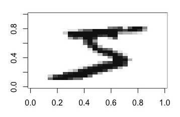
Each pixel represents an input, and each pixel is given a grayscale number, meaning a white pixel is 0, and a darker pixel is a number representing how dark the pixel is.
So, we input 784 values. These values are weighted (weights are learned through training data) and passed to the next layer of the network. A network and its layers look like this:
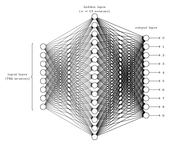
Each of the 784 input values is sent to each of the nodes in the middle (hidden) layer. What I mean by this is that one pixel value is sent to each of the 30 nodes in the hidden layer. In our case, this represents a 784 by 30 matrix as you’ll see we use 30 nodes in the hidden layer. You’ll also notice 10 nodes in what is called the output layer. Each of these nodes represents a final determination of the handwritten digit being 0 through 9.
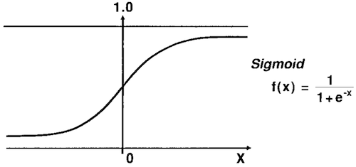
Let’s talk through how one pixel (input) would pass through the entire network after having been weighted and passed to the middle (hidden) layer. From here, the new, weighted value is input into the middle layer. The node in the middle layer takes the value and runs it through what is called an activation function. In our case, we’ll use a Sigmoid function which looks like this:
In R, our now weighted input is passed into the below function as z:
sigmoid <- function(z) 1/(1+exp(-z))So what does the Activation (Sigmoid) function do? In laymen’s terms, it determines if the input is of value. You’ll see what this means in the next paragraph.
From here, the output of the Sigmoid function is weighted and passed as input into the final layer of 10 nodes (remember: representing each of the 10 digits 0 through 9). That input is ran through the Activation function again, and the neural network outputs a vector of ten values, like this:
> a
              [,1]
 [1,] 0.1041222329
 [2,] 0.0056134030
 [3,] 0.3600190030
 [4,] 0.9930337436
 [5,] 0.0004073771
 [6,] 0.0179073440
 [7,] 0.0938795106
 [8,] 0.0071585077
 [9,] 0.9863697174
[10,] 0.0175402033
These values represent how much the neural network “thinks” the handwritten inputted image is each number. We simply take the highest output (closest to 1) and consider the neural network to have classified the digit as that value. This output is from an untrained network, but it makes logical sense that the network thinks an 8 and 3 look similar. In this case, we’d say the network predicts that the handwritten image is a 3!
The key points to remember of how a network classifies a digit are: edges weight the inputs, nodes determine if those weighted inputs are of value, the values at the nodes are passed on to be weighted and valued again until the output layer is reached. The output tells us what the input should be classified as.
Implementing NN in R
Now that we’ve briefly walked through what steps a network takes to classify a handwritten digit, we must walk through how we train the network to get good at classifying digits correctly.
To train a network, we must give it some data so it can learn. We do this by splitting the dataset. In our handwritten image dataset we have 70,000 images, so we’ll feed our network 60,000 images to learn from and 10,000 to test on. The primary difference between the “learning” and “testing” digits is that in the learning phase we are able to adjust the weights and biases such that it gets more digits right. This is done through a reduction in what is called a cost function.
Stochastic Gradient Descent
To start, we begin with the Stochastic Gradient Descent function. Gradient descent is a fancy way of saying we minimize the cost function (i.e. minimize how many digit classifications we get wrong). We want to minimize cost because cost represents how poorly our network classifies digits. The higher the cost, the worse our network classifies digits correctly.
The stochastic portion of Stochastic Gradient Descent references the fact that we are estimating gradient descent. We estimate it because we use mini batching — splitting the training data into mini-batches of size 10 (meaning each mini batch has 10 handwritten images in it):
training_data <- cbind(train$x, train$y)
for (j in 1:epochs) {
  training_data <- training_data[sample(nrow(training_data)), ]
  mini.batches <- list()
  seq1 <- seq(from = 1, to = 60000, by = mini.batch.size)
  for (u in 1:(nrow(training_data) / mini.batch.size)) {
    mini.batches[[u]] <- training_data[seq1[u]:(seq1[u] + 9), ]
  }
We create a nested list of 6000 mini batches, each of size mini.batch.size = 10.
Update Mini Batch
Within this function, we instantiate an empty list for the weights and biases and iterate through each observation in the mini batch, calling backpropagation for each:
nabla.b <- list(rep(0, sizes[2]), rep(0, sizes[3]))
nabla.w <- list(
  matrix(rep(0, (sizes[2] * sizes[1])), nrow = sizes[2], ncol = sizes[1]),
  matrix(rep(0, (sizes[3] * sizes[2])), nrow = sizes[3], ncol = sizes[2])
)
for (p in 1:mini.batch.size) {
  x <- mini_batch[p, -785]
  y <- mini_batch[p, 785]
  delta_nablas <- backprop(x, y, sizes, num_layers, biases, weight)
Backpropagation
Backpropagation takes the observations of a mini batch and determines the weights and biases that would correctly classify each digit. We feed observations forward first, calculating what our current network would classify the digit as:
activation <- matrix(x, nrow = length(x), ncol = 1)
activations <- list(matrix(x, nrow = length(x), ncol = 1))
zs <- list()

for (f in 1:length(weight)) {
  b <- biases[[f]]
  w <- weight[[f]]
  z <- w %*% activation + b
  zs[[f]] <- z
  activation <- sigmoid(z)
  activations[[f + 1]] <- activation
}
Then we backpropagate — determining the weights that would minimize the cost for this mini batch:
delta <- cost.derivative(activations[[length(activations)]], y) * sigmoid_prime(zs[[length(zs)]])
nabla_b_backprop[[length(nabla_b_backprop)]] <- delta
nabla_w_backprop[[length(nabla_w_backprop)]] <- delta %*% t(activations[[length(activations) - 1]])
The cost.derivative function subtracts 1 from the activation at the correct digit position — this is how the network learns what to correct:
cost.derivative <- function(output.activations, y) {
  output.activations - digit.to.vector(y)
}
Epochs
After iterating through all 6,000 mini batches (one epoch), we’ll have ~50% accuracy on the test set. The real improvement comes from repeating this process many times (epochs), incrementally tuning weights toward optimality. Banks automating check processing use this same principle — kind of cool, right?
In Closing
If you’ve made it this far, congratulations. I hope you’ve learned a little bit about how neural networks are implemented and how they learn. If you’d like to try it out for yourself, see the source code. There are a number of helper functions I didn’t go over for the sake of brevity, so be sure to familiarize yourself with those too. Otherwise, leave a comment below and let me know what you thought of this project!